
Population growth curvesSpec C4.1.7, C4.1.8
In short
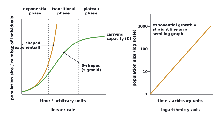
Population growth curves model how numbers change over time. When resources are plentiful and limiting factors are absent, a population grows exponentially, giving a J-shaped curve. As density-dependent factors take effect, growth slows and numbers level off at the carrying capacity, giving a sigmoid (S-shaped) curve. Exponential growth plots as a straight line on a logarithmic scale.
Exponential growth
In the first phase, when a few individuals colonise a new area, numbers increase exponentially: the population doubles at regular intervals. Reasons: resources are abundant, so there is little competition; predators, pathogens and parasites are scarce or absent; so the birth rate greatly exceeds the death rate, and every new individual soon adds offspring of its own.
Case study: in 1937, eight ring-necked pheasants (two males and six females) were released on Protection Island, Washington, USA, which had plenty of food and few predators. The population grew roughly exponentially, to more than 1300 birds after five years, before growth slowed. A second case: 29 reindeer released on St Matthew Island, Alaska, in 1944 grew to about 6000 by 1963. Having overgrazed their lichen food supply, almost all of them starved in the severe winter of 1963–64, and only 42 were alive in 1966, showing that exponential growth cannot continue.
Sigmoid growth
- Exponential phase: rapid increase, birth rate far greater than death rate.
- Transitional phase: density-dependent factors begin to act; the rate of increase slows but numbers still rise.
- Plateau phase: births plus immigration balance deaths plus emigration; the population fluctuates around the carrying capacity.
 (opens full size in a new tab)
To test whether growth is exponential, plot population size on a logarithmic vertical axis against time on a normal horizontal axis. Exponential growth gives a straight line; the line bends and flattens as growth slows towards the carrying capacity.
The sigmoid curve is an idealised model. Real populations overshoot, oscillate or crash, and their carrying capacity changes from year to year. Models are simplifications of complex systems, useful for making predictions and for comparison with real data.
Model sigmoid growth with duckweed (Lemna): count fronds in a beaker of pond water every 2–3 days. Or use yeast in sugar solution: count cells in a haemocytometer, or measure cloudiness with a colorimeter, at regular intervals. Keep temperature and light constant.
The IB sigmoid curve starts with exponential growth: a lag phase is not expected. Do not add a death phase either; that belongs to a closed culture running out of resources.
Written and checked against the IB Biology HL specification · Updated October 2026